OSMnx: Python for Street Networks

If you use OSMnx in your work, please cite the journal article.

Note that this blog post is not updated with every new release of OSMnx. For the latest, see the official documentation and usage examples.

OSMnx is a Python package to retrieve, model, analyze, and visualize street networks from OpenStreetMap. Users can download and model walkable, drivable, or bikeable urban networks with a single line of Python code, and then easily analyze and visualize them. You can just as easily download and work with amenities/points of interest, building footprints, elevation data, street bearings/orientations, and network routing. If you use OSMnx in your work, please download/cite the paper here.

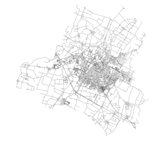
In a single line of code, OSMnx lets you download, model, and visualize the street network for, say, Modena Italy:

import osmnx as ox
ox.plot_graph(ox.graph_from_place('Modena, Italy'))

Installing OSMnx

OSMnx is on GitHub and you can install it with conda. If you’re interested in OSMnx but don’t know where to begin, check out this guide to getting started with Python.

OSMnx features

Check out the documentation and usage examples for details on using each of the following features:

• Download street networks anywhere in the world with a single line of code
• Download other infrastructure types, place boundaries, building footprints, and points of interest
• Download by city name, polygon, bounding box, or point/address + network distance
• Download drivable, walkable, bikeable, or all street networks
• Download node elevations and calculate edge grades (inclines)
• Impute missing speeds and calculate graph edge travel times
• Simplify and correct the network’s topology to clean-up nodes and consolidate intersections
• Fast map-matching of points, routes, or trajectories to nearest graph edges or nodes
• Save networks to disk as shapefiles, GeoPackages, and GraphML
• Save/load street network to/from a local .osm xml file
• Conduct topological and spatial analyses to automatically calculate dozens of indicators
• Calculate and visualize street bearings and orientations
• Calculate and visualize shortest-path routes that minimize distance, travel time, elevation, etc
• Visualize street network as a static map or interactive leaflet web map
• Visualize travel distance and travel time with isoline and isochrone maps
• Plot figure-ground diagrams of street networks and/or building footprints

How to use OSMnx

There are many usage examples and tutorials in the examples repo. I’ll demonstrate 5 basic use cases for OSMnx in this post:

1. Automatically download administrative place boundaries and shapefiles
2. Download and model street networks
3. Correct and simplify network topology
4. Save street networks to disk as shapefiles, GraphML, or SVG
5. Analyze street networks: routing, visualization, and calculating network stats

1. Get administrative place boundaries and shapefiles

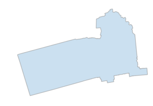
To acquire administrative boundary GIS data, one must typically track down shapefiles online and download them. But what about for bulk or automated acquisition and analysis? There must be an easier way than clicking through numerous web pages to download shapefiles one at a time. With OSMnx, you can download place shapes from OpenStreetMap (as geopandas GeoDataFrames) in one line of Python code - and project them to UTM (zone calculated automatically) and visualize in just one more line of code:

import osmnx as ox
city = ox.geocode_to_gdf('Berkeley, California')
ax = ox.project_gdf(city).plot()
_ = ax.axis('off')

You can just as easily get other place types, such as neighborhoods, boroughs, counties, states, or nations - any place geometry in OpenStreetMap:

place1 = ox.geocode_to_gdf('Manhattan, New York City, New York, USA')
place2 = ox.geocode_to_gdf('Cook County, Illinois')
place3 = ox.geocode_to_gdf('Iowa, USA')
place4 = ox.geocode_to_gdf('Bolivia')

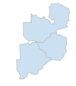
Or you can pass multiple places into a single query to save a single shapefile or geopackage from their geometries. You can do this with cities, states, countries or any other geographic entities:

places = ox.geocode_to_gdf(['Botswana', 'Zambia', 'Zimbabwe'])
places = ox.project_gdf(places)
ax = places.plot()
_ = ax.axis('off')

2. Download and model street networks

To acquire street network GIS data, one must typically track down Tiger/Line roads from the US census bureau, or individual data sets from other countries or cities. But what about for bulk, automated analysis? And what about informal paths and pedestrian circulation that Tiger/Line ignores? And what about street networks outside the United States? OSMnx handles all of these uses.

OSMnx lets you download street network data and build topologically-corrected street networks, project and plot the networks, and save the street network as SVGs, GraphML files, or shapefiles for later use. The street networks are directed and preserve one-way directionality. You can download a street network by providing OSMnx any of the following (demonstrated in the examples below):

• a bounding box
• a lat-long point plus a distance
• an address plus a distance
• a polygon of the desired street network’s boundaries
• a place name or list of place names

You can also specify several different network types:

• ‘drive’ - get drivable public streets (but not service roads)
• ‘drive_service’ - get drivable public streets, including service roads
• ‘walk’ - get all streets and paths that pedestrians can use (this network type ignores one-way directionality)
• ‘bike’ - get all streets and paths that cyclists can use
• ‘all’ - download all (non-private) OSM streets and paths
• ‘all_private’ - download all OSM streets and paths, including private-access ones

You can download and construct street networks in a single line of code using these various techniques:

2a) street network from bounding box

This gets the drivable street network within some lat-long bounding box, in a single line of Python code, then projects it to UTM, then plots it:

G = ox.graph_from_bbox(37.79, 37.78, -122.41, -122.43, network_type='drive')
G_projected = ox.project_graph(G)
ox.plot_graph(G_projected)

You can get different types of street networks by passing a network_type argument, including driving, walking, biking networks (and more).

2b) street network from lat-long point

This gets the street network within 0.75 km (along the network) of a latitude- longitude point:

G = ox.graph_from_point((37.79, -122.41), dist=750, network_type='all')
ox.plot_graph(G)

You can also specify a distance in cardinal directions around the point, instead of along the network.

2c) street network from address

This gets the street network within 1 km (along the network) of the Empire State Building:

G = ox.graph_from_address('350 5th Ave, New York, New York', network_type='drive')
ox.plot_graph(G)

You can also specify a distance in cardinal directions around the address, instead of along the network.

2d) street network from polygon

Just load a shapefile with geopandas, then pass its shapely geometry to OSMnx. This gets the street network of the Mission District in San Francisco:

G = ox.graph_from_polygon(mission_shape, network_type='drive')
ox.plot_graph(G)

2e) street network from place name

Here’s where OSMnx shines. Pass it any place name for which OpenStreetMap has boundary data, and it automatically downloads and constructs the street network within that boundary. Here, we create the driving network within the city of Los Angeles:

G = ox.graph_from_place('Los Angeles, California', network_type='drive')
ox.plot_graph(G)

You can just as easily request a street network within a borough, county, state, or other geographic entity. You can also pass a list of places (such as several neighboring cities) to create a unified street network within them. This list of places can include strings and/or structured key:value place queries:

places = ['Los Altos, California, USA',
    {'city':'Los Altos Hills', 'state':'California'},
    'Loyola, California']
G = ox.graph_from_place(places, network_type='drive')
ox.plot_graph(G)

2f) street networks from all around the world

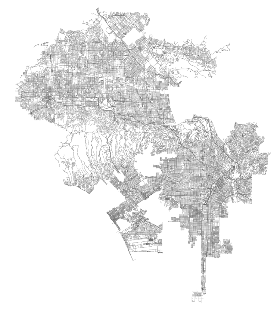
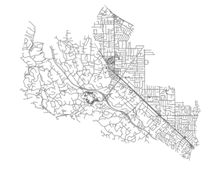
In general, US street network data is fairly easy to come by thanks to Tiger/Line shapefiles. OSMnx makes it easier by making it available with a single line of code, and better by supplementing it with all the additional data from OpenStreetMap. However, you can also get street networks from anywhere in the world - places where such data might otherwise be inconsistent, difficult, or impossible to come by:

G = ox.graph_from_place('Modena, Italy')
ox.plot_graph(G)

G = ox.graph_from_place('Belgrade, Serbia')
ox.plot_graph(G)

G = ox.graph_from_address('Maputo, Mozambique', distance=3000)
ox.plot_graph(G)

G = ox.graph_from_address('Bab Bhar, Tunis, Tunisia', distance=3000)
ox.plot_graph(G)

3. Correct and simplify network topology

Note: you can also topologically consolidate nearby intersections.

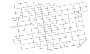
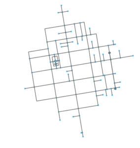
Simplification is done by OSMnx automatically under the hood, but we can break it out to see how it works. OpenStreetMap nodes can be weird: they include intersections, but they also include all the points along a single street segment where the street curves. The latter are not nodes in the graph theory sense, so we remove them algorithmically and consolidate the set of edges between “true” network nodes into a single edge.

When we first download and construct the street network from OpenStreetMap, it looks something like this:

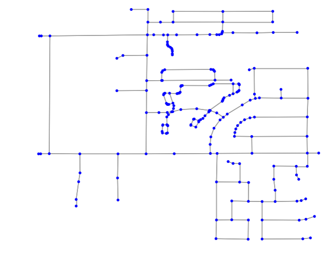
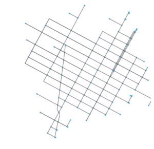
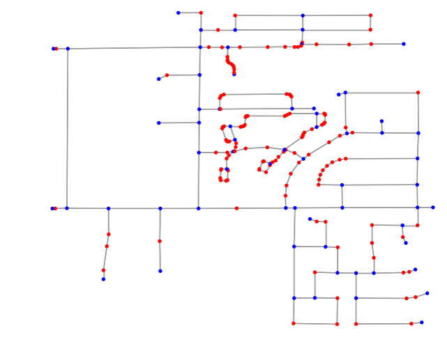
We want to simplify this network to only retain the nodes that represent the junction of multiple streets. OSMnx does this automatically. First it identifies all non-intersection nodes:

And then it removes them, but faithfully maintains the spatial geometry of the street segment between the true intersection nodes:

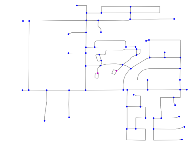
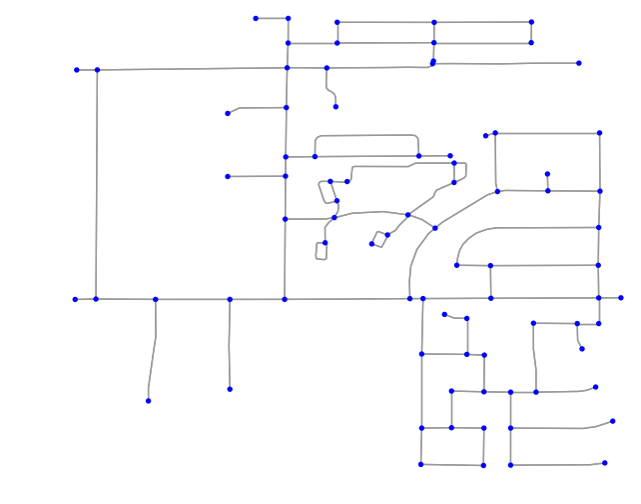
Above, all the non-intersection nodes have been removed, all the true intersections (junctions of multiple streets) remain in blue, and self-loop nodes are in purple. There are two simplification modes: strict and non- strict. In strict mode (above), OSMnx considers two-way intersections to be topologically identical to a single street that bends around a curve. If you want to retain these intersections when the incident edges have different OSM IDs, use non-strict mode:

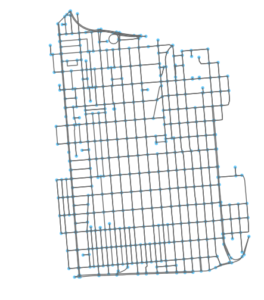
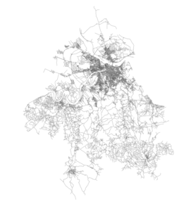
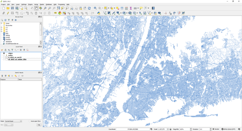
4. Save street networks to disk

OSMnx can save the street network to disk as a GraphML file to work with later in Gephi or networkx. Or it can save the network (such as this one, for the New York urbanized area) as ESRI shapefiles or GeoPackages to work with in any GIS:

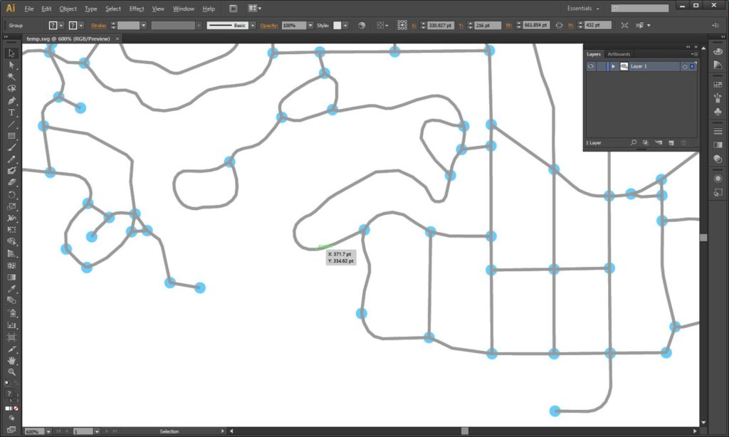
OSMnx can also save street networks as SVG files for design work in Adobe Illustrator:

You can then load any network you saved as GraphML back into OSMnx to calculate network stats, solve routes, or visualize it.

5. Analyze street networks

Since this is the whole purpose of working with street networks, I’ll break analysis out in depth in a future dedicated post. But I’ll summarize some basic capabilities briefly here. OSMnx is built on top of NetworkX, geopandas, and matplotlib, so you can easily analyze networks and calculate spatial network statistics:

G = ox.graph_from_place('Santa Monica, California', network_type='walk')
basic_stats = ox.basic_stats(G)
print(basic_stats['circuity_avg'])
extended_stats = ox.extended_stats(G, bc=True)
print(extended_stats['betweenness_centrality_avg'])

The stats are broken up into two primary functions: basic and extended. The extended stats function also has optional parameters to run additional advanced measures.

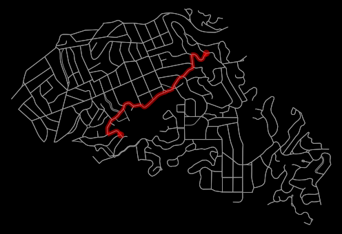
You can also calculate and plot shortest-path routes between points, taking one-way streets into account:

G = ox.graph_from_place('Piedmont, CA, USA', network_type='drive')
route = nx.shortest_path(G, orig, dest)
fig, ax = ox.plot_graph_route(G, route, route_linewidth=6, node_size=0, bgcolor='k')

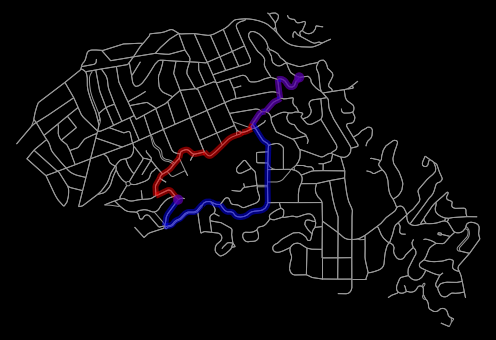
You can impute missing edge speeds and calculate edge travel times (see example) to contrast shortest paths by distance (red) vs by travel time (blue):

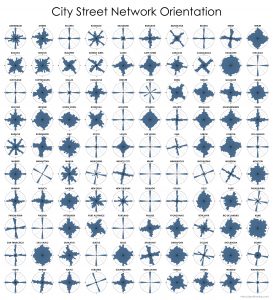
You can also visualize the compass orientation of street networks around the world:

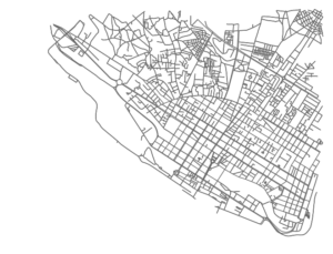
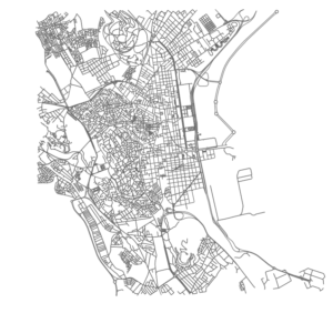
Allan Jacobs famously compared several cities’ urban forms through figure-ground diagrams of 1 square mile of each’s street network in his book Great Streets. We can re-create this automatically and computationally with OSMnx:

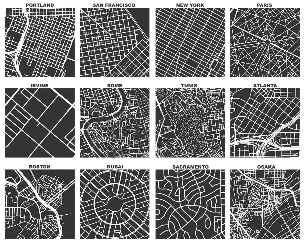
These figure-ground diagrams are created completely with OSMnx.

Conclusion

OSMnx lets you download spatial geometries and model, project, visualize, and analyze real-world street networks. It allows you to automate the data collection and computational analysis of street networks for powerful and consistent research, transportation planning, and urban design. OSMnx is built on top of NetworkX, matplotlib, and geopandas for rich network analytic capabilities, beautiful and simple visualizations, and fast spatial queries with r-tree, kd-tree, and ball-tree indexes.

OSMnx is open-source and on GitHub. You can download/cite the paper here.