Categories
Planning

City Street Orientations around the World

City street network grid orientations, order, disorder, entropy, rose plot, polar histogram made with Python, OSMnx, OpenStreetMap, matplotlib.This post is adapted from this research paper that you can read/cite for more info. It analyzes and visualizes 100 cities around the world.

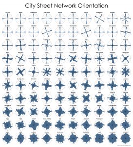
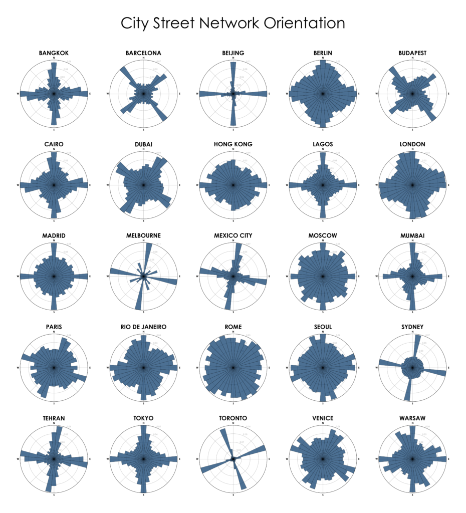
By popular request, this is a quick follow-up to this post comparing the orientation of streets in 25 US cities using Python and OSMnx. Here are 25 more cities around the world:

City street network grid orientations, rose plot, polar histogram made with Python, OSMnx, OpenStreetMap, matplotlib. Bangkok, Barcelona, Beijing, Budapest, Cairo, Delhi, Dubai, Glasgow, Hong Kong, Lagos, London, Madrid, Melbourne, Mexico City, Moscow, Mumbai, Munich, Paris, Rio de Janeiro, Rome, Seoul, Sydney, Tehran, Toronto, Warsaw, Tokyo, Berlin, Venice

Categories
Planning

Comparing US City Street Orientations

City street network grid orientations, order, disorder, entropy, rose plot, polar histogram made with Python, OSMnx, OpenStreetMap, matplotlib.This post is adapted from this research paper that you can read/cite for more info. It analyzes and visualizes 100 cities around the world.

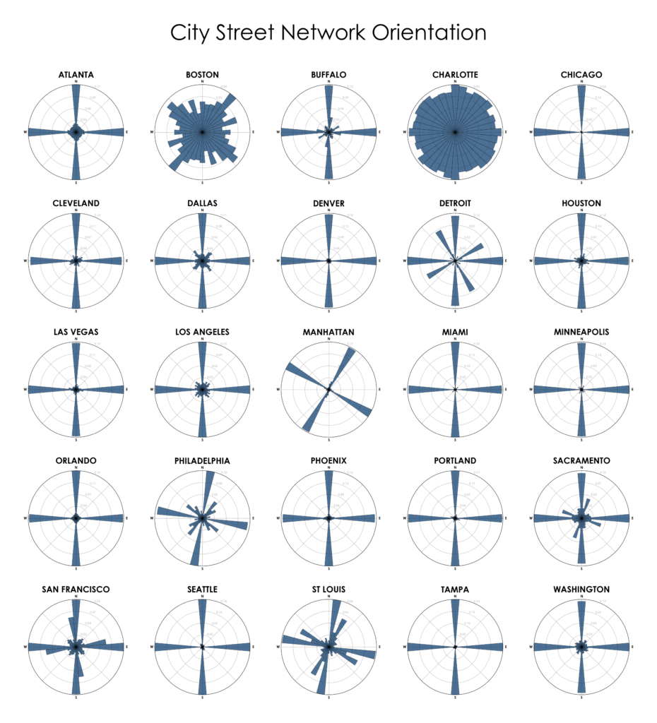
“We say the cows laid out Boston. Well, there are worse surveyors.” –Ralph Waldo Emerson. In 1960, one hundred years after Emerson’s quote, Kevin Lynch published The Image of the City, his treatise on the legibility of urban patterns. How coherent is a city’s spatial organization? How do these patterns help or hinder urban navigation? I recently wrote about visualizing street orientations with Python and OSMnx. That is, how is a city’s street network oriented in terms of the streets’ compass bearings? How well does it adhere to a straightforward north-south-east-west layout? I wanted to revisit this by comparing 25 major US cities’ orientations (EDIT: by popular request, see also this follow-up comparing world cities):

City street network grid orientations, rose plot, polar histogram made with Python, OSMnx, OpenStreetMap, matplotlib. Atlanta, Boston, Buffalo, Charlotte, Chicago, Cleveland, Dallas, Denver, Detroit, Houston, Las Vegas, Los Angeles, Manhattan, New York, Miami, Minneapolis, Orlando, Philadelphia, Phoenix, Portland, Sacramento, San Francisco, Seattle, St Louis, Tampa, Washington DC.

Categories
Planning

Estimating Daytime Density in RSRS

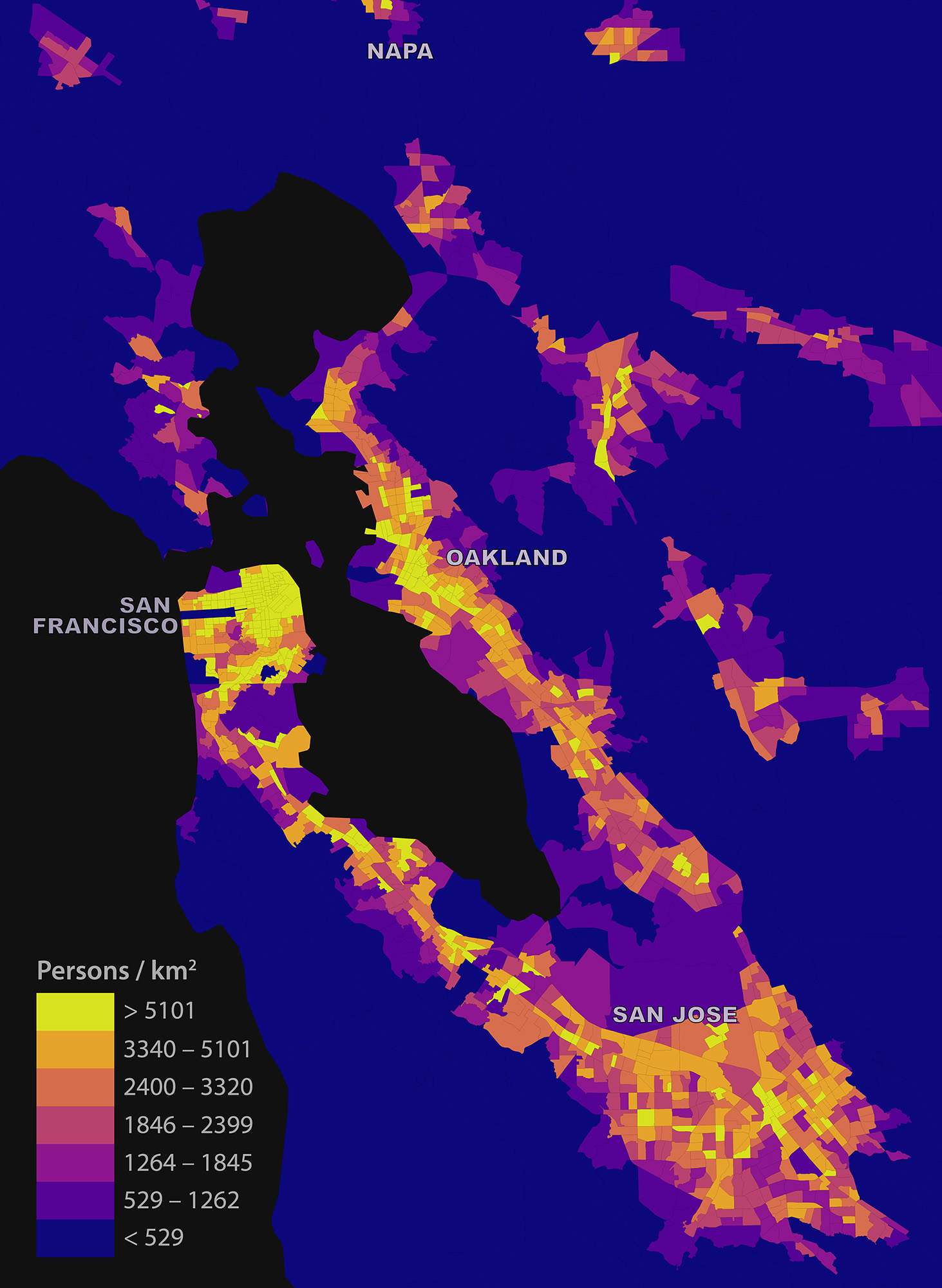
My short article “Estimating Local Daytime Population Density from Census and Payroll Data” is out now in the latest issue of Regional Studies, Regional Science. I discuss a method for estimating local daytime density across a metropolitan area using US Census and LEHD LODES data, and dig into some limitations and biases. I look at the San Francisco Bay Area as a case study:

Map of the estimated daytime population density in the San Francisco Bay Area

Categories
Data

Network-Based Spatial Clustering

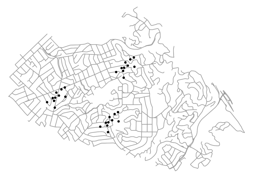
Jobs, establishments, and other amenities tend to agglomerate and cluster in cities. To identify these agglomerations and explore their causes and effects, we often use spatial clustering algorithms. However, urban space cannot simply be traversed as-the-crow-flies: human mobility is network-constrained. To properly model agglomeration along a city’s street network, we must use network-based spatial clustering.

The code for this example can be found in this GitHub repo. We use OSMnx to download and assemble the street network for a small city. We also have a dataframe of points representing the locations of (fake) restaurants in this city. Our restaurants cluster into distinct districts, as many establishments and industries tend to do:

firm locations on the street network to be clustered: python, osmnx, matplotlib, scipy, scikit-learn, geopandas

Categories
Data

OSMnx Features Round-Up

OSMnx is a Python package for quickly and easily downloading, modeling, analyzing, and visualizing street networks and other spatial data from OpenStreetMap. Here’s a quick round-up of recent updates to OSMnx. I’ll try to keep this up to date as a single reference source. A lot of new features have appeared in the past few months, and people have been asking about what’s new and what’s possible. You can:

  • Download and model street networks or other networked infrastructure anywhere in the world with a single line of code
  • Download any other spatial geometries, place boundaries, building footprints, or points of interest as a GeoDataFrame
  • Download by city name, polygon, bounding box, or point/address + network distance
  • Download drivable, walkable, bikeable, or all street networks
  • Download node elevations and calculate edge grades (inclines)
  • Impute missing speeds and calculate graph edge travel times
  • Simplify and correct the network’s topology to clean-up nodes and consolidate intersections
  • Fast map-matching of points, routes, or trajectories to nearest graph edges or nodes
  • Save networks to disk as shapefiles, geopackages, and GraphML
  • Save/load street network to/from a local .osm xml file
  • Conduct topological and spatial analyses to automatically calculate dozens of indicators
  • Calculate and visualize street bearings and orientations
  • Calculate and visualize shortest-path routes that minimize distance, travel time, elevation, etc
  • Visualize street networks as a static map or interactive leaflet web map
  • Visualize travel distance and travel time with isoline and isochrone maps
  • Plot figure-ground diagrams of street networks and building footprints
Categories
Data

Street Network Orientation

OSMnx is a Python package for easily downloading and analyzing street networks anywhere in the world. Among other analyses, we can use it to explore street network orientation. That is, what are the bearings and spatial orientations of the streets in the network? All of the code for this example is in this GitHub notebook. First we use OSMnx to download the street network of Moraga, California, a small town in the hills just east of Berkeley:

Moraga, California street network OSMnx OpenStreetMap Python

OSMnx automatically calculates all of the streets’ bearings. Specifically it calculates the compass bearing from each directed edge’s origin node u to its destination node v. Now we can visualize these bearings, binned together as a histogram to get a sense of the relative frequency of the streets’ spatial orientations. Or better yet, we can project that histogram as a polar plot to match the compass bearings:

Moraga, California street network orientation edge bearings polar plot OSMnx OpenStreetMap Python

Categories
Data

Urban Street Network Centrality

Check out the journal article about OSMnx.

We can measure and visualize how “important” a node or an edge is in a network by calculating its centrality. Lots of flavors of centrality exist in network science, including closeness, betweenness, degree, eigenvector, and PageRank. Closeness centrality measures the average shortest path between each node in the network and every other node: more central nodes are closer to all other nodes. We can calculate this easily with OSMnx, as seen in this GitHub demo. For example, here is the node closeness centrality for Piedmont, California:

Urban street network graph node closeness and betweenness centrality

Categories
Planning

Estimating Daytime Population Density

Check out the journal article about this project.

I was recently asked: “how might someone figure out the local daytime population density across the Bay Area from public data?” My answer, in short, was that you really couldn’t accurately. But you could at least produce a coarse, biased estimate. Here’s how.

I examined the Bay Area’s tract-level daytime population density using three input data products: the 2010 TIGER/Line census tracts shapefile with DP1 attributes, the 2010 California LEHD LODES data, and the census bureau’s 2010 US states shapefile. I preferred the 2010 census demographic data to (more recent) ACS data because the ACS tract-level variables are five-year rolling averages. Given this, I preferred not to compare 2014 LODES data to 2010-2014 ACS data as the Bay Area experienced substantial housing, economic, and demographic upheaval over this interval – patterns obscured in the ACS rolling average. To avoid inconsistent comparison, I opted for more stale – but more accurate and comparable – data.

Map of the estimated daytime population density in the San Francisco Bay Area

Categories
Academia

New Article: Craigslist Housing Markets in JPER

Our article “New Insights into Rental Housing Markets across the United States: Web Scraping and Analyzing Craigslist Rental Listings” is finally appearing in print in the Journal of Planning Education and Research‘s forthcoming winter issue. We collected, validated, and analyzed 11 million Craigslist rental listings to discover fine-grained patterns across metropolitan housing markets in the United States.

Map of 1.5 million Craigslist rental listings in the contiguous U.S., divided into quintiles by each listing's rent per square foot. Published in JPER: the Journal of Planning Education and Research.

Categories
Academia

New Article: OSMnx in CEUS

My article “OSMnx: New methods for acquiring, constructing, analyzing, and visualizing complex street networks” was published in the journal Computers, Environment and Urban Systems earlier this month. OSMnx is a Python package that lets you download a street network anywhere in the world at any scale with a single line of code, then analyze or visualize it with one more line of code.

OSMnx: Figure-ground diagrams of one square mile of each street network, from OpenStreetMap, made in Python with matplotlib, geopandas, and NetworkX