Network-Based Spatial Clustering

Jobs, establishments, and other amenities tend to agglomerate and cluster in cities. To identify these agglomerations and explore their causes and effects, we often use spatial clustering algorithms. However, urban space cannot simply be traversed as-the-crow-flies: human mobility is network-constrained. To properly model agglomeration along a city’s street network, we must use network-based spatial clustering.

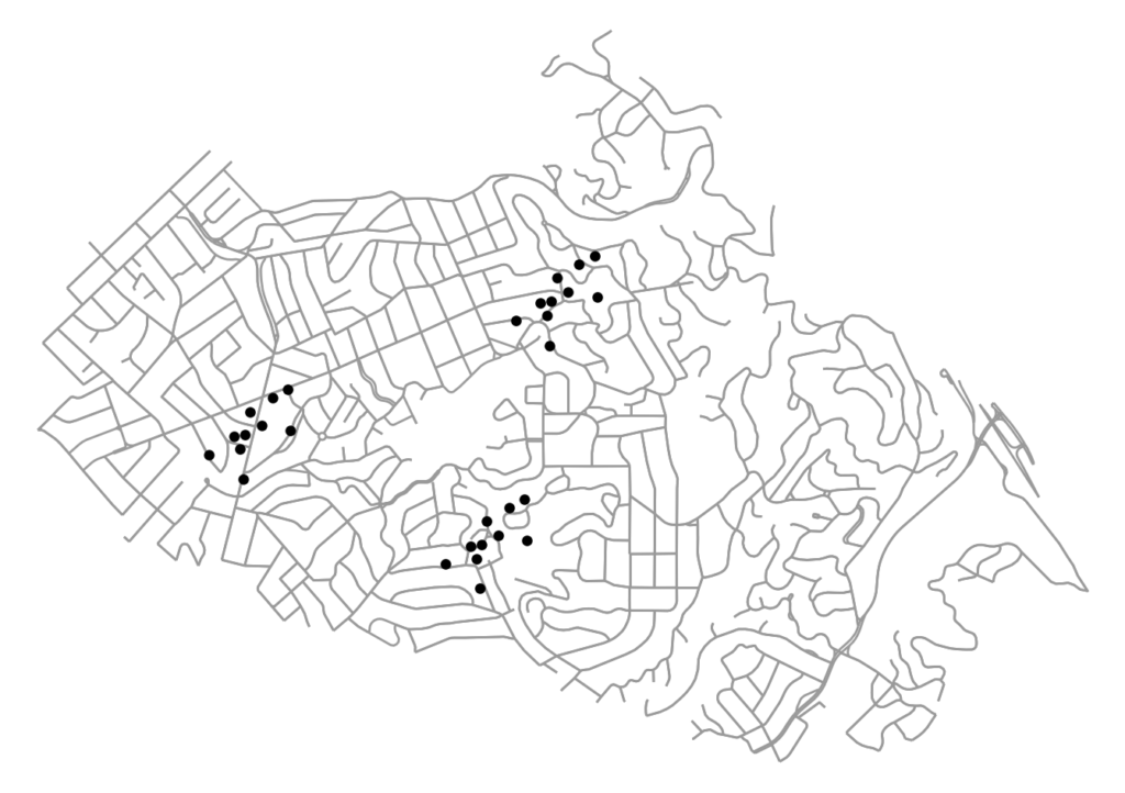
The code for this example can be found in this GitHub repo. We use OSMnx to download and assemble the street network for a small city. We also have a dataframe of points representing the locations of (fake) restaurants in this city. Our restaurants cluster into distinct districts, as many establishments and industries tend to do:

If we want to explore how these establishments agglomerate, we can identify spatial clusters using an algorithm like DBSCAN. DBSCAN identifies points as members of a cluster if each is within epsilon distance of another and if this cluster contains at least minpts number of points. For this example we parameterize it with an epsilon = 300 and minpts = 3. That is, points must be within 300 meters of each other and a cluster must contain at least 3 points. For more on DBSCAN, check out this blog post and paper.

We compute DBSCAN by converting everything to radians, fitting it, then getting cluster labels for each establishment:

eps_rad = 300 / 3671000. #meters to radians
db = DBSCAN(eps=eps_rad, min_samples=3, metric='haversine', algorithm='ball_tree')
df['spatial_cluster'] = db.fit_predict(np.deg2rad(df[['y', 'x']]))

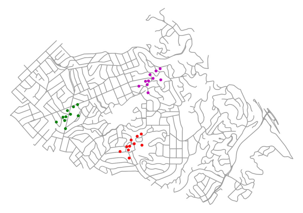
Now we can visualize our establishments, coloring them by spatial cluster label:

Our three clusters of establishments are clearly visible in red, magenta, and green, representing three distinct districts in the city. Each cluster contains at least 3 points and no point is more than 300 meters away from another. Except for one problem: in cities, we usually cannot travel as-the-crow-flies. Rather, urban circulation is constrained to networks of streets and paths. Due to terrain and other factors, even adjacent land parcels may not interface with each other except through a long trip along the street network.

The image above provides an example. The red cluster’s right-most 3 points lay on a street loop that does not directly connect to the rest of the cluster’s street network, due to the terrain. Although these two parts of the cluster are within our epsilon distance (300m) of each other spatially, they are much farther apart when traveling along the network, as you would have to do in reality.

To identify how these points cluster together in a meaningful way given that urban circulation is network-constrained, we must re-label them using network-based spatial clustering. First we use OSMnx to attach every establishment to its nearest network node:

df['nn'] = ox.get_nearest_nodes(G, X=df['x'], Y=df['y'], method='balltree')

Then we create a function to calculate a node-based network distance matrix:

def network_distance_matrix(u, G, vs=nodes_unique):
    dists = [nx.dijkstra_path_length(G, source=u, target=v, weight='length') for v in vs]
    return pd.Series(dists, index=vs)

Next we calculate the distance matrix using our OSMnx street network, G, and re-index to make the matrix establishment-based.

nodes_unique = pd.Series(df['nn'].unique())
nodes_unique.index = nodes_unique.values
node_dm = nodes_unique.apply(network_distance_matrix, G=G)
node_dm = node_dm.astype(int)

# reindex to create establishment-based net dist matrix
ndm = node_dm.reindex(index=df['nn'], columns=df['nn'])

Finally, we re-compute DBSCAN using the same parameters, but this time fitting it to our precomputed establishment-based network distance matrix (we can also use a sparse matrix to speed up computation – see notebook for an example):

db = DBSCAN(eps=300, min_samples=3, metric='precomputed')
df['network_cluster'] = db.fit_predict(ndm)

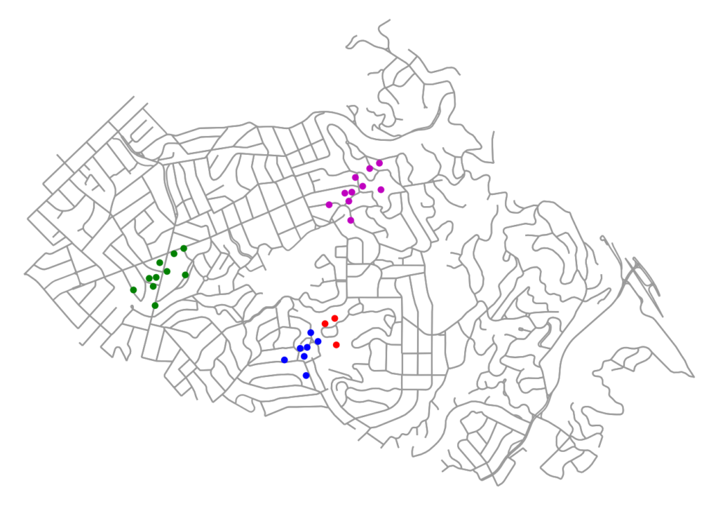
Now we visualize our establishments again, coloring them by network cluster label:

When clustered spatially earlier, we got 3 clusters. Now, when we do network-constrained density-based spatial clustering, we get 4 clusters: the formerly unified red cluster has now split into separate red and blue clusters that cannot reach one another within 300 meters along the network. This more accurately reflects circulation and agglomeration in real-world urban space, which is network-constrained.

All of the code to re-create this network clustering workflow is in this Jupyter notebook in this GitHub repo. For a more complicated example clustering millions of points along a network, see this notebook. For more on using DBSCAN for spatial clustering, compression, and dimensionality reduction see this blog post and paper.