In a previous post I discussed how to reduce the size of a spatial data set by clustering. Too many data points in a visualization can overwhelm the user and bog down on-the-fly client-side map rendering (for example, with a javascript tool like Leaflet). So, I used the DBSCAN clustering algorithm to reduce my data set from 1,759 rows to 158 spatially-representative points. This series of posts discusses this data set in depth.
The Douglas-Peucker algorithm
Today I’ll show another method for reducing the size of a spatial data set in Python using the shapely package’s implementation of the Douglas-Peucker algorithm. Douglas-Peucker reduces the number of points in a curve composed of line segments by recursively dividing the line. The final result is a subset of points from the original curve.
All of my code is available in this GitHub repo, particularly this IPython notebook. Let’s begin. First I import the necessary modules and load the full data set:
import pandas as pd, numpy as np, matplotlib.pyplot as plt
from shapely.geometry import LineString
from time import time
df = pd.read_csv('summer-travel-gps-full.csv')
coordinates = df.as_matrix(columns=['lat', 'lon'])
Next, I create a shapely LineString from the coordinate data. This is the curve that will comprise line segments between the coordinate points. I will then simplify the geometry of this curve using shapely’s simplify method.
If preserve topology is set to False, the method will use the Douglas-Peucker algorithm, which is fine – I don’t need to preserve topology because I just need a reduced set of points. I also specify a tolerance value. All points in the simplified figure will be within the tolerance distance of the original geometry. After running the algorithm, I’ll print out a couple of descriptive stats to see what I ended up with:
line = LineString(coordinates)
tolerance = 0.015
simplified_line = line.simplify(tolerance, preserve_topology=False)
print len(line.coords), 'coordinate pairs in full data set'
print len(simplified_line.coords), 'coordinate pairs in simplified data set'
print round(((1 - float(len(simplified_line.coords)) / float(len(line.coords))) * 100), 1), 'percent compressed'
1759 coordinate pairs in full data set
178 coordinate pairs in simplified data set
89.9 percent compressed
The Douglas-Peucker algorithm reduced the size of the data set by about 90%, from 1,759 data points in the original full set to 178 points in the new reduced data set. That’s not bad – these stats are comparable to results from clustering. Now let’s save the simplified set of coordinates as a new pandas dataframe:
lon = pd.Series(pd.Series(simplified_line.coords.xy)[1])
lat = pd.Series(pd.Series(simplified_line.coords.xy)[0])
si = pd.DataFrame({'lon':lon, 'lat':lat})
si.tail()
           lat        lon
173  41.044556  28.983285
174  41.008992  28.968268
175  41.043487  28.985488
176  40.977637  28.823879
177  48.357110  11.791346
Find matching points in the original data set
The original full data set was reverse-geocoded and included city/country data and timestamps. The simplified set however only contains coordinate lat-long data. So, I’ll write a short routine that, for each row in the simplified set, finds the row label of the row that contains its matching lat-long coordinates in the original full set.
First I add a new column to the simplified set to contain the index of the matching row from the original full data set. Then for each row in the simplified set I loop through each row in the original full set, comparing tuples of coordinates. If the points match, I save this full set row’s index as the match in the new column I added to the simplified set. It’s simpler than it sounds:
start_time = time()
si['df_index'] = None
for si_i, si_row in si.iterrows():
    si_coords = (si_row['lat'], si_row['lon'])
    for df_i, df_row in df.iterrows():
        if si_coords == (df_row['lat'], df_row['lon']):
            si['df_index'][si_i] = df_i
            break
print 'process took %s seconds' % round(time() - start_time, 2)
process took 5.37 seconds
Now I select the rows from the original full data set whose indices appear in the df_index column of the simplified data set. Then I save the data set to CSV and examine its tail:
rs = df.ix[si['df_index'].dropna()]
rs.to_csv('summer-travel-gps-simplified.csv', index=False)
rs.tail()
            lat        lon              date      city  country
1730  41.044556  28.983285  07/08/2014 16:44  Istanbul   Turkey
1739  41.008992  28.968268  07/08/2014 20:03  Istanbul   Turkey
1745  41.043487  28.985488  07/08/2014 22:18  Istanbul   Turkey
1751  40.977637  28.823879  07/09/2014 09:03  Istanbul   Turkey
1758  48.357110  11.791346  07/09/2014 13:20    Munich  Germany
Looks good! I now have 178 rows of the original full data set, with city/country data and timestamps.
Comparing the full vs reduced data sets
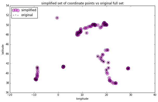
Let’s plot the new simplified set of GPS coordinate data against the original full set:
plt.figure(figsize=(10, 6), dpi=100)
rs_scatter = plt.scatter(rs['lon'], rs['lat'], c='m', alpha=.4, s=150)
df_scatter = plt.scatter(df['lon'], df['lat'], c='k', alpha=.3, s=10)
plt.xlabel('longitude')
plt.ylabel('latitude')
plt.title('simplified set of coordinate points vs original full set')
plt.legend((rs_scatter, df_scatter), ('simplified', 'original'), loc='upper left')
plt.show()
The new reduced data set closely approximates the spatial distribution of the original full data set. You can compare it to the results I got by clustering: the Douglas-Peucker gave us a better reduced data set than the k-means clustering algorithm did, and one comparable to result of the DBSCAN clustering algorithm.
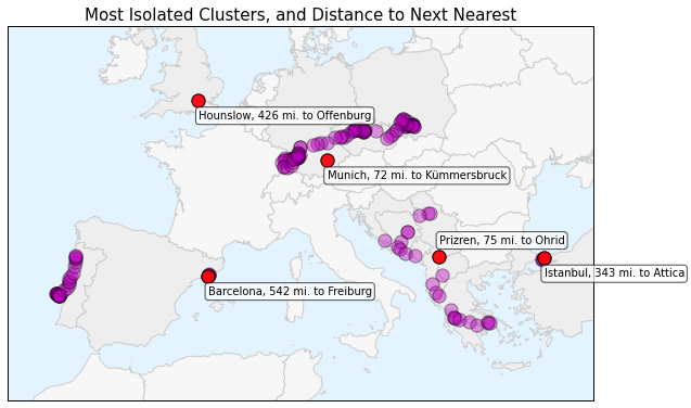
Now you can visualize the data set in more interesting ways:

